Variational State-Space Models for Localisation and Dense 3D Mapping in 6 DoF
Scaling generative spatial models to the real world
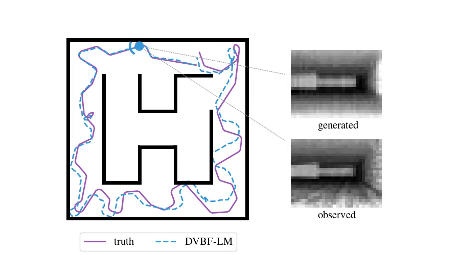
In a previous post, we saw how useful spatial models are for navigating and exploring new environments. There we introduced a probabilistic model called DVBF-LM, targeting simulated 2D setups. Let us now think about a drone flying in 3D space and viewing the world through an RGB-D camera. How do we localise it mid-flight? How do we reconstruct a consistent map of everything it has seen so far? How do we predict its video stream for the next ten seconds of flight?
These are central questions when controlling moving agents. They address state estimation and prediction, two major pillars needed for decision making. In this post we will go over one way to solve these challenges. For this, we will pick up where we left off last time and modify the assumptions of the DVBF-LM model, scaling it to real-world data.
Background
First we recap the framework we will use. We denote the RGB-D video stream our agent perceives over time with \(\obs\Ts\). These are our observations. The collected images are fused into a map representation \(\map\). In parallel we estimate the history of agent states \(\state\Ts\) from which the images were recorded. The map and the states are latent (meaning, we cannot measure them), so we need to infer them. This all comes together in the following probabilistic graphical model:
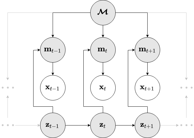
Or put in math, the joint distribution of all variables is:
This matches the generative factorisation of our previous DVBF-LM (please check the new paper (Mirchev et al., 2021) or the preceding blog post for the details). In short, images are formed by first attending locally to the map with \(p(\chart\t \mid \state\t, \map)\) (deterministic) and then sculpting the extracted \(\chart\t\) into an observation with \(p(\obs\t \mid \chart\t)\).
If you scan the above equation, you will also notice the control inputs \(\control\Tsm\). We model their influence through a dynamics model \(p_{\genpars_T}(\state\tp \mid \state\t, \control\t)\). This lets us imagine how the agent would move and what it would see for certain controls and plan its next actions accordingly. We will come back to this later.
Motivation behind the modelling changes
So why are changes to DVBF-LM necessary in the first place? Let's look at the requirements:
- Localisation and mapping need to happen on-the-fly in unknown environments.
- We want real-world 3D representations and models of 6-DoF agent movement.
- We want geometric consistency of the predicted images from novel viewpoints.
- We want sufficient accuracy and efficiency.
A real-world model demands a 3D map, and DVBF-LM's map is a 2D grid. We also want to capture free 6-DoF agent movement, and in DVBF-LM the poses are bound to a plane, \(\state = (x, y, \theta)\). With these obvious limitations out of the way, we are left with a more intricate challenge – ensuring geometric consistency. Unsurprisingly, the crux is in the map, attention and emission. Consider the following schematic depiction:
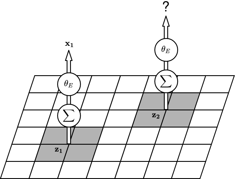
The left picture shows how DVBF-LM constructs observations \(\obs\). The 2D grid is a map with abstract content. DVBF-LM's attention takes only the four cells underneath the state \(\state\), which are then transformed into an observation \(\obs\) by an MLP (= a multi-layer perceptron aka a neural network). Modulo some details, the construction of observations is a black box to us, due to the unidentified map information and the MLP.
There are two major issues with this. First, the attention is too narrow. When the map learns to reconstruct \(\obs_1\), it updates the cells undeneath \(\state_1\), but when we go to \(\state_2\) we have no knowledge of what is there, even if \(\state_2\) was already in the field of view of \(\state_1\). Such redundancy is inefficient. Second, even with a broader attention geometric consistency is not guaranteed: the content stored under \(\state_1\) has no controlled effect on the observation predicted at \(\state_2\), due to the MLP: it could have learned any transformation.
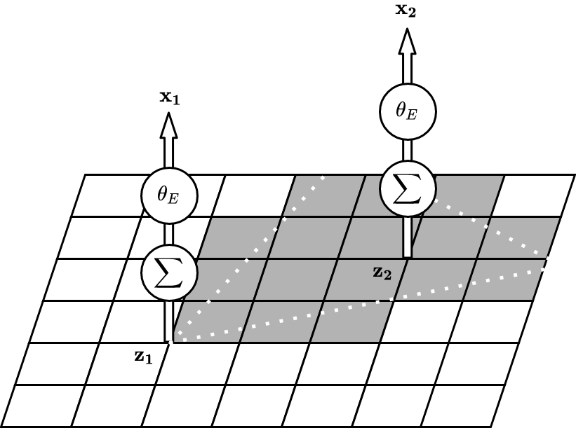
Enforcing geometric consistency in a black-box model through learning alone is an arduous task. With real-world scenes and images comes the curse of dimensionality. Universal generalisation would require large volumes of data, and we want inference of the map and states to happen on-the-fly.
So how about injecting some domain knowledge, just enough to make the black box more transparent? We depict this on the right above – we can attend to the exact field-of-view of our sensor. We can use identified map content that we understand, such as occupancy, so that we can engineer how geometry works and thus make sure that emitting from \(\state_2\) will be consistent with \(\state_1\). While this means more work for us, the designers, it does not limit how expressive the model is. This is because our understanding of geometry is exact, and we do not sacrifice much when that concept is not learned from data.
The assumptions
In summary, we only preserve the graphical model of DVBF-LM. We change all the building blocks, following the motivation above: the states \(\state\Ts\), the map \(\map\), the attention \(p(\chart\t \mid \state\t, \map)\), the emission \(p(\obs\t \mid \chart\t)\), the transition \(p_{\genpars_T}(\state\tp \mid \state\t, \control\t)\) and the approximate posterior \(q_\varpars(\state\Ts, \map)\) are all new.
Changes in the generative model
The states \(\state\) now represent a 6-DoF pose (location, orientation) and also track linear velocity.
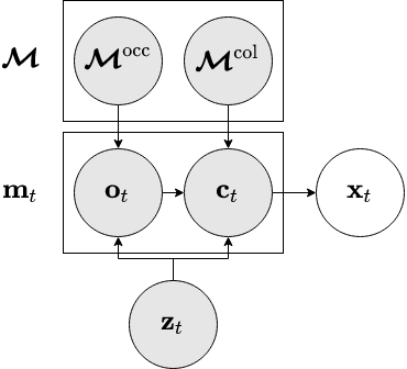 The map consists of an occupancy grid \(\mapocc\) and a neural network \(\mapcol\).
Both of these take a point from \(\mathbb{R}^3\) as input, and predict the occupancy and colour at that point, respectively.
The map consists of an occupancy grid \(\mapocc\) and a neural network \(\mapcol\).
Both of these take a point from \(\mathbb{R}^3\) as input, and predict the occupancy and colour at that point, respectively.
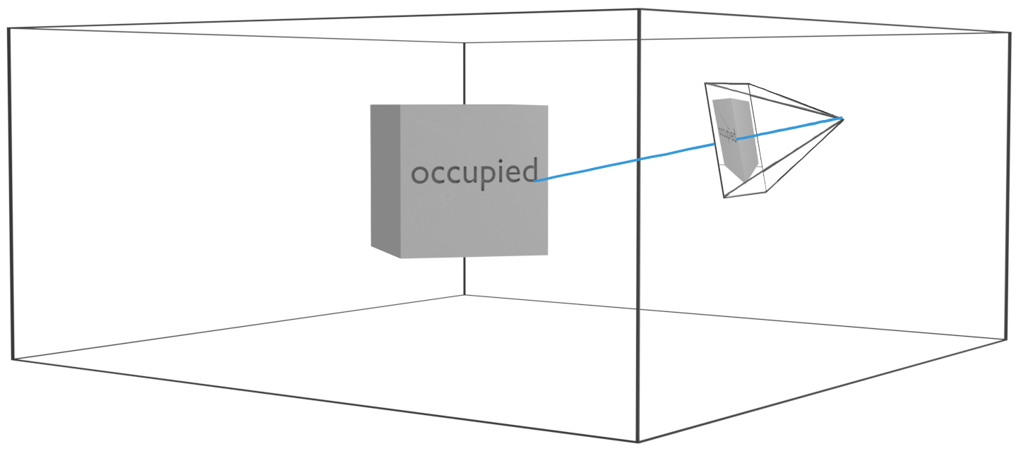
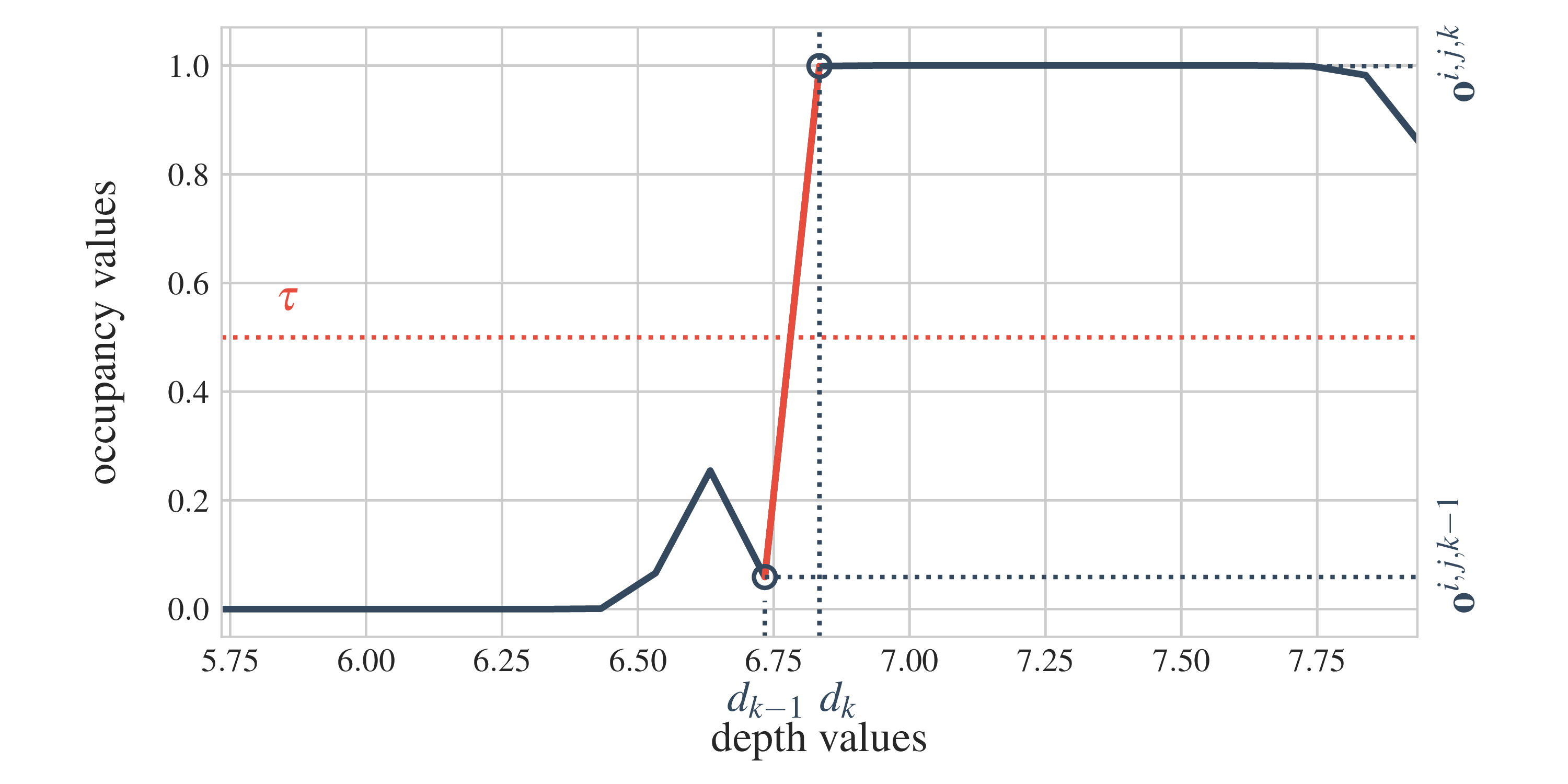
The attention \(p(\chart\t \mid \state\t, \map)\) is simply the camera frustum. Rays are projected for every image pixel, and the map content is extracted for a set of discrete points along each ray. The extracted map chart thus consists of a volume of occupancy and a volume of colour: \(\chart = (\chartocc, \chartcol)\) (see figure on the right).
The RGB-D images are then sculpted by first finding the first occupancy hit along each ray in \(\chartocc\), and then determining the respective depth and colour (corresponding entry from \(\chartcol\)) for that hit position. In total the conditionals \(p(\chart\t \mid \state\t, \map)\) and \(p(\obs\t \mid \chart\t)\) define a differentiable rendering procedure, as shown in the next image.
With proper 6-DoF poses and 3D occupancy and colour representations we can simulate real scenes. The geometric consistency of rendered observations is ensured through the attention that respects the camera's field of view and the explicit volumetric raycasting based on occupancy. On a side note, this is the same set of assumptions that underpin NERF (Mildenhall et al., 2020), which is compatible with our framework.
Changes in the approximate posterior
Particle filters as in DVBF-LM don't scale well to the state dimensionality we need. We opt for non-amortised inference of the states and the map:
with free variational parameters for every \(\state_t\) and \(\map\). We leave amortisations in the state posterior as interesting future work. The parameters are inferred with SGD, as our model is end-to-end differentiable.
Learning drone dynamics
We want a strong predictive dynamics model. We model the transition as a residual MLP on top of engineered Euler dynamics \(f_T\):
This way the model is initialised close to the engineered integration in the beginning of training, and the MLP has freedom to take over and correct for biases present in the control stream. We learn it from prerecorded MOCAP data of agent movement using a secondary variational state-space model. You can take the details from the paper. Its predictions look like this (in orange):

Bridging the gap between generative models and traditional SLAM
It is worth noting that multiple-view geometry assumptions similar to the inductive biases we introduce are at the heart of traditional visual odometry and simultaneous localisation and mapping (SLAM) systems (DurrantWhyte et al. (1996); Cadena et al. (2016)). Historically, the focus of SLAM has been entirely on inference of the map and poses, targeting very accurate localisation. Our model brings accurate inference to the domain of spatial generative models (Fraccaro et al. (2018); Mirchev et al. (2019)), that additionally act as simulators of the mapped environment and can predict agent movement and observations with uncertainty. The posterior approximation
is the equivalent of SLAM in this model, and the predictive generative model \(p(\state_{2:T}, \obs\Ts \mid \control\Tsm, \state_1)\) is something we gain on top, perfectly aligned with the SLAM inference.
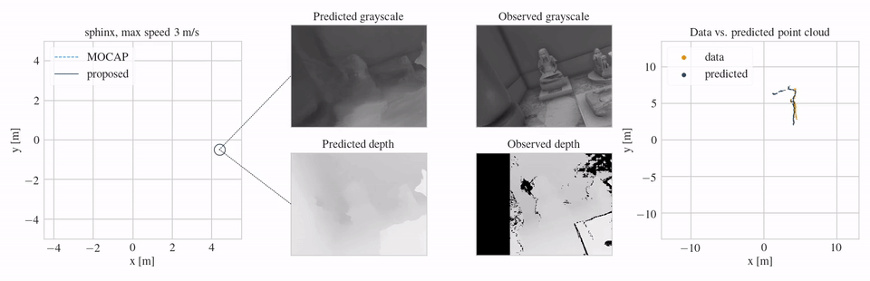
Localisation and mapping
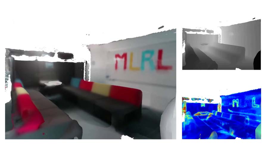
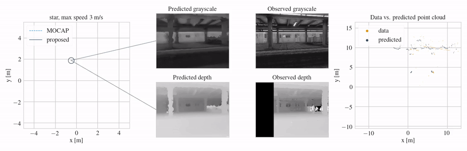
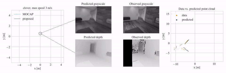
With the revised model, we can now successfully localise a real drone in a variety of different environments. We can also reconstruct dense maps in the process. You can see this in the following three videos: localisation on the left, image reconstructions from the learned map in the middle and a top-down view of a predicted point cloud on the right. Notice how the predicted point cloud is filtering the observed noise.
Predicting ahead
What is more, beside SLAM inference we also have a predictive distribution \(p(\state_{2:T}, \obs\Ts \mid \control\Tsm, \state_1)\). This is something not readily available in most traditional SLAM systems. This model lets us predict how the agent would move and what it would see for a future sequence of control inputs.
Remember how I mentioned the controls would be of importance – well, this is where they come into the picture. We can imagine what would happen to the system if we'd move, and this is the main prerequisite for enabling planning and control.
The next video first shows mean inference estimates for the past in blue, followed by prediction samples for the future in orange. Notice how the model offers uncertainty when predicting ahead.
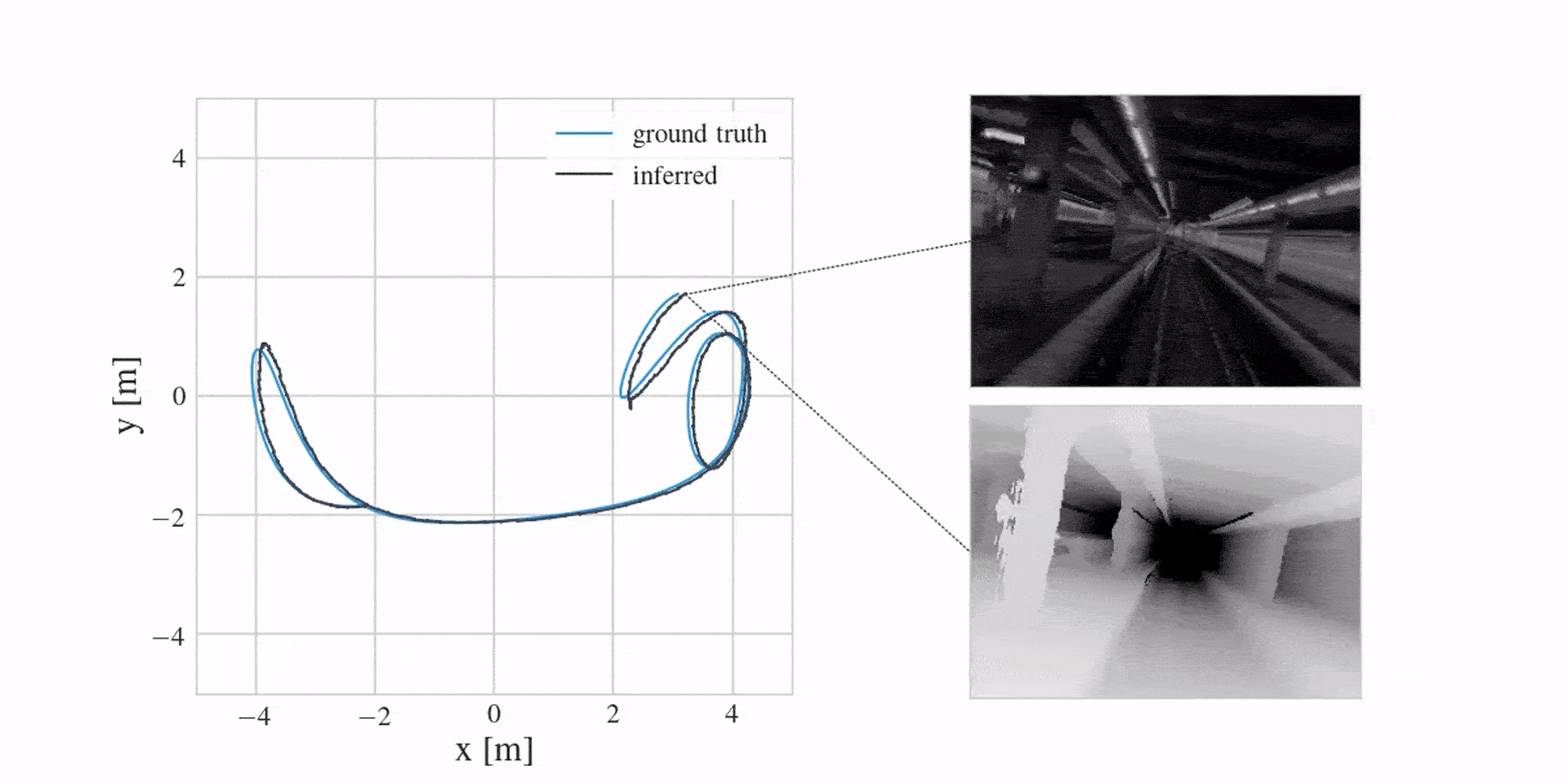
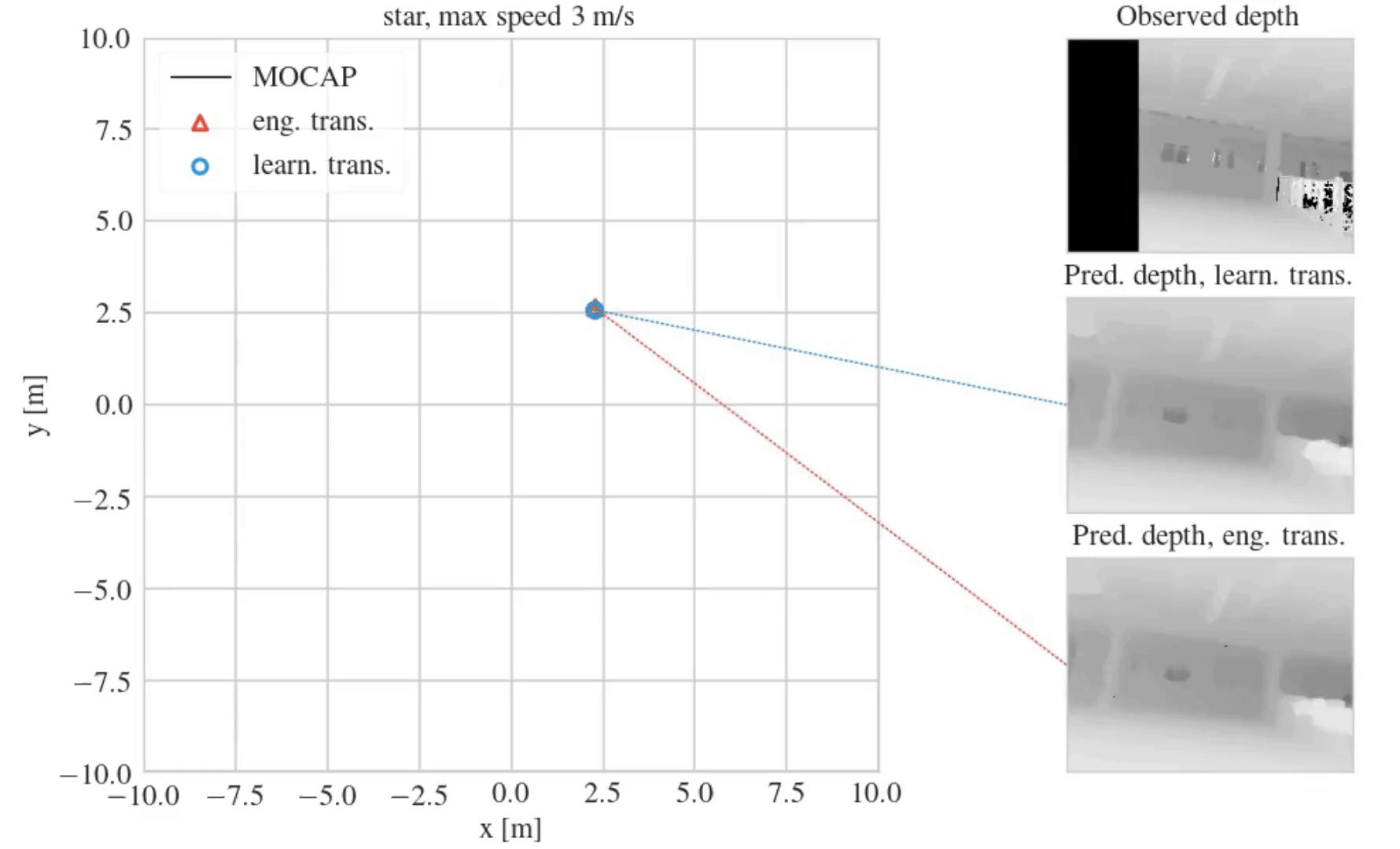
And in case you were wondering if learning a corrective MLP in the dynamics model is better than engineering everything, the following video shows this (here we see mean depth predictions):
Collision modelling
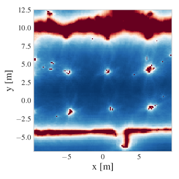 With the aforementioned predictive model at hand we can evaluate different cost-to-go functions (value functions) for optimal control and reinforcement learning.
Here we briefly illustrate this with a computed collision cost-to-go along a 2D slice of a reconstructed NYC Subway Station environment from the Blackbird data set (Antonini et al., 2020).
As one would expect, the collision cost-to-go is high at the obstacles (walls, pillars), and gradually drops off in the free space.
With the aforementioned predictive model at hand we can evaluate different cost-to-go functions (value functions) for optimal control and reinforcement learning.
Here we briefly illustrate this with a computed collision cost-to-go along a 2D slice of a reconstructed NYC Subway Station environment from the Blackbird data set (Antonini et al., 2020).
As one would expect, the collision cost-to-go is high at the obstacles (walls, pillars), and gradually drops off in the free space.
TL;DR
- Injecting domain knowledge from multiple-view geometry and rigid-body dynamics allows us to scale generative spatial models to the real world.
- This does not limit the learning flexibility of the system, as everything remains fully differentiable and probabilistic.
- With the variational-inference framework, we perfectly align SLAM inference with a probabilistic predictive model.
- The predictive model is then useful for downstream simulation for planning and control.
- Learning a corrective MLP for the dynamics in the predictive model leads to better long-term predictions than after engineering everything by hand.
The presented model is a significant step-up from DVBF-LM. It is almost as accurate as traditional SLAM methods and offers a rich predictive distribution for the simulation of real-world scenarios. What is left is to improve the runtime, such that it can be deployed on real hardware. We are excited about the prospects of applying model-based reinforcement learning and control with it.
Stay tuned!
This work was published at the International Conference on Learning Representations (ICLR), 2021. We refer to the paper for a more detailed discussion: OpenReview, preprint.
Bibliography
Amado Antonini, Winter Guerra, Varun Murali, Thomas Sayre-McCord, and Sertac Karaman. The blackbird uav dataset. The International Journal of Robotics Research, 0(0):0278364920908331, 2020. arXiv:https://doi.org/10.1177/0278364920908331, doi:10.1177/0278364920908331. ↩
Cesar Cadena, Luca Carlone, Henry Carrillo, Yasir Latif, Davide Scaramuzza, José Neira, Ian D. Reid, and John J. Leonard. Past, present, and future of simultaneous localization and mapping: toward the robust-perception age. IEEE Trans. Robotics, 32(6):1309–1332, 2016. ↩
Hugh Durrant-Whyte, David Rye, and Eduardo Nebot. Localization of autonomous guided vehicles. In Georges Giralt and Gerhard Hirzinger, editors, Robotics Research, 613–625. London, 1996. Springer London. ↩
Marco Fraccaro, Danilo Jimenez Rezende, Yori Zwols, Alexander Pritzel, S. M. Ali Eslami, and Fabio Viola. Generative temporal models with spatial memory for partially observed environments. CoRR, 2018. arXiv:1804.09401. ↩
Ben Mildenhall, Pratul P. Srinivasan, Matthew Tancik, Jonathan T. Barron, Ravi Ramamoorthi, and Ren Ng. Nerf: representing scenes as neural radiance fields for view synthesis. In ECCV. 2020. ↩
Atanas Mirchev, Baris Kayalibay, Maximilian Soelch, Patrick van der Smagt, and Justin Bayer. Approximate Bayesian inference in spatial environments. In Proceedings of Robotics: Science and Systems. Freiburg im Breisgau, Germany, June 2019. doi:10.15607/RSS.2019.XV.083. ↩
Atanas Mirchev, Baris Kayalibay, Patrick van der Smagt, and Justin Bayer. Variational state-space models for localisation and dense 3d mapping in 6 dof. In International Conference on Learning Representations. 2021. URL: https://openreview.net/forum?id=XAS3uKeFWj. ↩