Spatial World Models
Tracking and Planning in 3D
Can we scale world models to real-life environments? Our latest work uses spatial world models to power real-time pose inference and planning.
This post is the latest installment in a series focusing on spatial environments. For earlier parts, see: Part 1, on Bayesian inference in spatial environments, and Part 2, on variational state-space models.
World models have been among the most exciting avenues of machine-learning research in recent years. These approaches combine traditional model-based reasoning with deep learning, leading to algorithms that are able to reason about the dynamics of complex systems and use that information with robust planning algorithms (to name a few notable works: Hafner et al. (2021), BeckerEhmck et al. (2020), Ha and Schmidhuber (2018)). For all their merits, these approaches fall short in learning good world models with few data and minimal human intervention. There are exciting developments in this area, e.g. a recent paper by Wu et al. (2022) shows that a four-legged robot can learn to walk within an hour using model-based reinforcement learning. Still, the same algorithm struggles with a task like visual navigation, requiring two hours to reach a fixed goal within a small obstacle-free area — insufficient from autonomous acting in real-world spaces.
Today, our most advanced world models are able to learn simple robot dynamics and small scenes in computer games. Can we extend our methods to understand real-world living spaces such as office floors or apartments?
We have been following this question for the past five years. Our initial, humble attempts were able to capture simple cartoon environments:
This method and its contemporaries (e.g. work by Fraccaro et al. (2018)) relied heavily on deep learning, which put hard requirements on the amount of data that was necessary to learn a good model. Data sets of real-world environments are scarce and of limited scope and do not match the richness of real spaces. We needed algorithms that were capable of acting in a new environment with as little data as possible. We needed inductive biases.
In our follow-up work we drew from recent advances in differentiable rendering and neural radience fields (Mildenhall et al. (2020)). These methods use information about 3D geometry to create emission functions that closely resemble raytracing. Structuring our generative models in this way finally allowed capturing the complexity of the real world, leading to an algorithm that could do simultaneous localisation and mapping in large, realistic spaces with drones.
Yet, something was still missing: speed. Continuously estimating the agent's pose with a NERF-like model came at a high cost. We needed faster inference to meet our ultimate goal of real-time autonomous acting. Our most recent work adds two more missing pieces of the puzzle: real-time tracking and planning.
Efficient inference with differentiable renderers
Camera pose inference with differentiable renderers relies on optimising the likelihood of observations through gradient descent:
Following the notation of our earlier posts, \(\obs,\state,\control\) and \(\map\) denote an RGB-D observation, an agent state, a control command and the environment map (which has been learned from a data set of camera poses and images, see Part 2 for more on this). This objective uses the current guess about the agent's state to render an RGB-D image, then compares that to the actual observation and optimises the agent's state so that the two match. The problem here is that rendering an image is expensive. Related work deals with this by subsampling the image with a small number of pixels (as done by Sucar et al. (2021) and YenChen et al. (2021)). We show a method that is as accurate while being four times faster. The crux of our method is to replace the likelihood \(\log p(\obs \mid \state, \map)\) with a proxy objective:
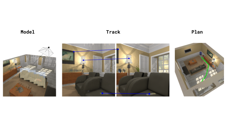
This expression looks quite a bit more complicated, but it has a simple intuitive explanation. Given a new observation in the form of an RGB-D image, we first pick an anchor pose (\(\state_{t-1}^*\) above). This is typically the most recent estimate of the camera pose. We render an RGB-D image from the anchor pose using the model. We start with some initial guess of the current camera pose, e.g. this might be the anchor pose with some small additive noise. We then optimise this guess by projecting pixels from the camera observation into the rendered anchor image using 3D geometry (denoted by \(\pi(\transform_{\state_{t}}^{\state_{t-1}^*}\point_{t}^k)\) above). The two terms in the objective are then simply the RGB and depth errors of these pixels in the projected image (except that the "depth error" is actually calculated using surface normals \(\hat\normal_{t-1}^k\) estimated from the depth).
This procedure is not new and is commonly known as point-to-plane ICP with photometric constraints (Chen and Medioni (1992), Steinbrucker et al. (2011), Audras et al. (2011)). It has been applied in other areas before, but we are the first to use it in the context of differentiable rendering. The most important difference of the point-to-plane objective to the likelihood objective is that rendering only has to be done once for the anchor pose, before optimisation begins. The anchor pose and its rendered image are kept fixed throughout optimisation, unlike the likelihood objective which has to render at every gradient step.
We extend the point-to-plane objective minimally, to allow using agent dynamics. The idea is that we usually have some coarse estimate of the agent's motion based on control commands that were used, which comes in the form of a transition model \(p(\state_{t+1}\mid\state_t,\control_t)\). This model is used as an additive term:
This objective is four times faster to optimise with no compromise in accuracy when compared to an analogous objective that relies on optimising through the renderer:
Here is a break-down of accuracy and speed:
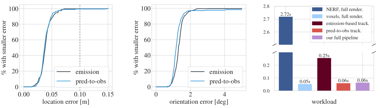
The first two panels show cumulative distribution functions of the location and orientation errors, taken over a set of representative localisation trials. In black is the method that optimises through the renderer and in blue our approach. We see that the two methods make errors in the same exact way. The final panel is a break-down of the run times involved in both approaches. The crimson bar in the centre shows the cost of optimising through the renderer with pixel subsampling. The next bar is the run time of our approach. Our method is able to run at 16 Hz realtime, while the baseline is limited to 4 Hz.
Planning with Spatial World Models
The next step is to use our learned model and real-time tracking method in an autonomous decision-making pipeline. We keep things as simple as possible and use an A*-planner. Here's an overview of our full pipeline:
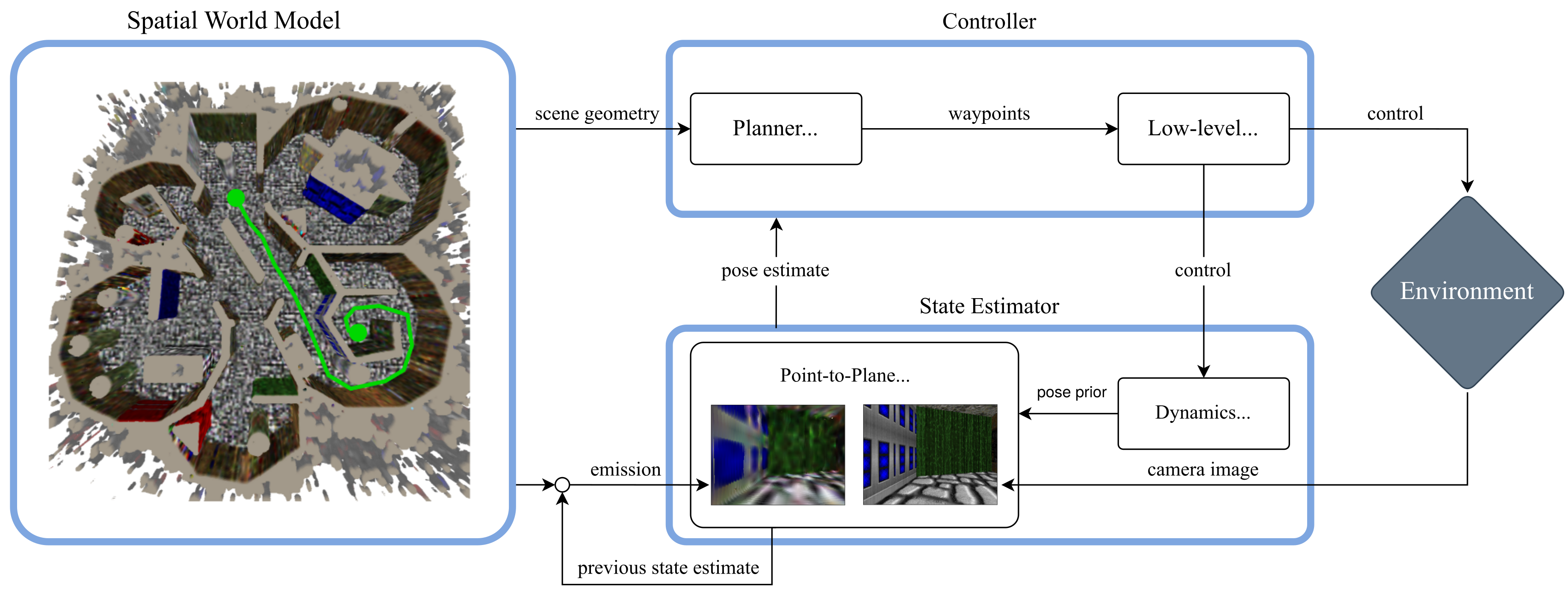
An environment model is learned from an data set of camera poses and RGB-D images. The model contains a colour map and an occupancy map, which are voxel grids. The occupancy map is used by an A*-planner which returns a set of landmarks that the agent must follow. Following the plan can be done with a simple low-level controller assuming the agent has the dynamics of a unicycle.
Evaluating our Approach
We want our approach to work in a diverse set of realistic environments and under noise. To that end we convert six realistic floor plans into levels for the ViZDoom simulator (Wydmuch et al. (2018)).
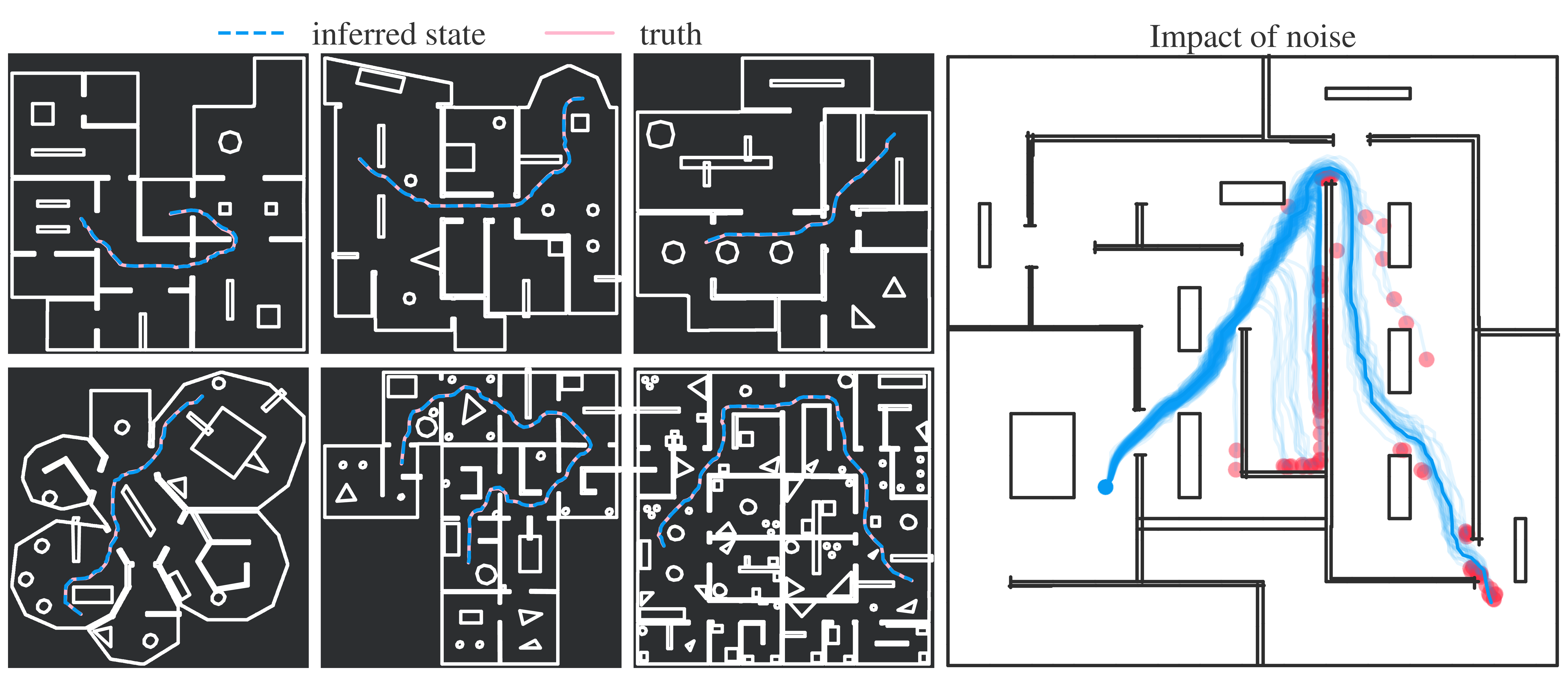
Since we rely on simulated environments for experiments, adding some form of noise to the agent's actions is important to get a better feeling of our method's true performance. Simulated environments lack disruptive factors that would come into play on real hardware. Adding noise helps approximate such factors, though it is not the same as testing in the real world. We experiment with different levels of noise, the effects of which can be seen in the final panel on the right. Executing the same actions (from the dark blue curve) under different random perturbations leads to vastly different outcomes, which makes it necessary to track the pose of the agent and re-plan actions.
In the highest noise setting, the noise can be quite disruptive to the agent, acting as an adversary that both hinders the agent's movement and throws off the tracker:
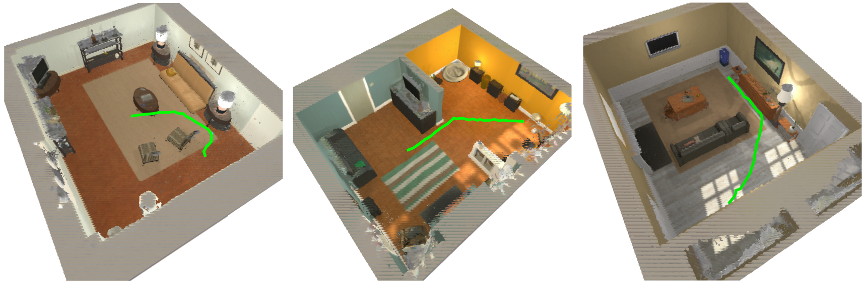
This is an example from the AI2-THOR simulator (Kolve et al. (2017)) which we use for additional qualitative experiments, since ViZDoom's visual fidelity is limited.
For evaluating navigation performance, we use the success weighted by path length (SPL) metric proposed by Anderson et al. (2018). This has a simple definition:
Given a set of navigation tasks \(\mathcal{S}\), we check for each one if it was successful (denoted by the flag \(s_i\)) and calculate the ratio of the length of the optimal path (\(l_i\)) to the length of the path that the agent took (\(p_i\)). SPL is between \(0\) and \(1\), where a value of \(1\) corresponds to an agent that always reaches the target using the optimal path.
We repeat our evaluation under three noise settings: low, medium and high. Our approach obtains SPL values of 0.92, 0.79 and 0.46 in these settings. Crucially, using a spatial world model always outperforms baselines that rely on dynamics alone and baselines which only use observations without a world model.
We test how well our method extends to environments that are more visually realistic than ViZDoom using the AI2-THOR simulator. Our spatial world models can capture the complexity of this higher-fidelity setup:
We have come a long way in spatial world models, but our work is not finished. A central assumption in this work was that the world model is learned from a limited offline dataset. The next piece of the puzzle will be to relax this assumption, enabling fully autonomous acting in entirely new scenes.
Until next time!
This work was published at the Learning for Dynamics and Control conference (L4DC), 2022, by Baris Kayalibay, Atanas Mirchev, Patrick van der Smagt and Justin Bayer. Please read the original paper and supplementary material.
Bibliography
Peter Anderson, Angel Chang, Devendra Singh Chaplot, Alexey Dosovitskiy, Saurabh Gupta, Vladlen Koltun, Jana Kosecka, Jitendra Malik, Roozbeh Mottaghi, Manolis Savva, and Amir R. Zamir. On evaluation of embodied navigation agents. 2018. arXiv:1807.06757. ↩
Cedric Audras, A Comport, Maxime Meilland, and Patrick Rives. Real-time dense appearance-based slam for rgb-d sensors. In Australasian Conf. on Robotics and Automation, volume 2, 2–2. 2011. ↩
Philip Becker-Ehmck, Maximilian Karl, Jan Peters, and Patrick van der Smagt. Learning to fly via deep model-based reinforcement learning. 2020. URL: https://arxiv.org/abs/2003.08876, arXiv:2003.08876. ↩
Yang Chen and Gérard Medioni. Object modelling by registration of multiple range images. Image and vision computing, 10(3):145–155, 1992. ↩
Marco Fraccaro, Danilo Jimenez Rezende, Yori Zwols, Alexander Pritzel, S. M. Ali Eslami, and Fabio Viola. Generative temporal models with spatial memory for partially observed environments. CoRR, 2018. arXiv:1804.09401. ↩
David Ha and Jürgen Schmidhuber. World models. CoRR, 2018. URL: http://arxiv.org/abs/1803.10122, arXiv:1803.10122. ↩
Danijar Hafner, Timothy Lillicrap, Mohammad Norouzi, and Jimmy Ba. Mastering atari with discrete world models. 2021. arXiv:2010.02193. ↩
Eric Kolve, Roozbeh Mottaghi, Winson Han, Eli VanderBilt, Luca Weihs, Alvaro Herrasti, Daniel Gordon, Yuke Zhu, Abhinav Gupta, and Ali Farhadi. AI2-THOR: An Interactive 3D Environment for Visual AI. arXiv, 2017. ↩
Ben Mildenhall, Pratul P. Srinivasan, Matthew Tancik, Jonathan T. Barron, Ravi Ramamoorthi, and Ren Ng. Nerf: representing scenes as neural radiance fields for view synthesis. In ECCV. 2020. ↩
Frank Steinbrücker, Jürgen Sturm, and Daniel Cremers. Real-time visual odometry from dense rgb-d images. In 2011 IEEE international conference on computer vision workshops (ICCV Workshops), 719–722. IEEE, 2011. ↩
Edgar Sucar, Shikun Liu, Joseph Ortiz, and Andrew J. Davison. Imap: implicit mapping and positioning in real-time. 2021. arXiv:2103.12352. ↩
Philipp Wu, Alejandro Escontrela, Danijar Hafner, Ken Goldberg, and Pieter Abbeel. Daydreamer: world models for physical robot learning. 2022. URL: https://arxiv.org/abs/2206.14176, doi:10.48550/ARXIV.2206.14176. ↩
Marek Wydmuch, Michał Kempka, and Wojciech Jaśkowski. Vizdoom competitions: playing doom from pixels. IEEE Transactions on Games, 2018. ↩
Lin Yen-Chen, Pete Florence, Jonathan T. Barron, Alberto Rodriguez, Phillip Isola, and Tsung-Yi Lin. Inerf: inverting neural radiance fields for pose estimation. 2021. arXiv:2012.05877. ↩