Approximate Bayesian inference in spatial environments
How to reason about space and moving agents
Knowledge about the state of a system is the basis for its control. For a robot arm, this can well be the joint angle sensors, and possibly its tactile sensor or camera input. For a mobile agent, however, such as a drone, it is the sensory observation of the space around it, as well as an understanding of that space. In practice: a map, with, of course, its location on that map.
This post discusses a probabilistic platform designed to learn and represent a map of physical space. A spatially-aware agent needs to know where it is (localisation) based on what it has seen before, and how it has moved. It also needs to know the position of things around it (mapping). Following our understanding of how to efficiently do machine learning, we frame both of these as probabilistic inference. With that base, we solve two more tasks through the same unified model: navigating from point A to point B and exploring unseen environments.
Probabilistic localisation and mapping
The task of Simultaneous Localisation and Mapping (SLAM), first coined by DurrantWhyte et al. (1996), makes up the first part of our problem. Imagine the following setup: over time, an agent is moving about and observing its surroundings. It is recording what it sees in a sequence \(\obs\Ts\). This can, for example, be a sequence of camera images or laser distance measurements. The agent needs to figure out its own pose \(\pose\Ts\) over time and a global world map \(\map\). It has to do so solely by looking at the history of observations \(\obs\Ts\) and controls \(\control\Ts\).
SLAM can be defined as a probabilistic inference problem. To do this, we treat \(\obs\Ts, \pose\Ts\) and \(\map\) as random variables. The goal is to find the posterior:
To solve this, we frame the problem probabilistically. For once, the framework is extensible—in the future we can add more interesting variables and infer them just like \(\pose\Ts\) and \(\map\). We can also pose additional objectives based on uncertainty estimates—we can define robust methods; this is also how we define exploration below.
In pursuit of better models: our objective
SLAM models consist of multiple components (or functions): modelling how an agent moves with \(\pose\tp = f(\pose\t)\), modelling how an observation \(\obs_t\) would be generated with \(\obs\t = f(\pose\t,\map)\), etc. In traditional implementations, an engineer specifies these functions based on hand-crafted world models. To simplify that task, the functions are often linearised, leading to a simpler and tractable model —typically using Kalman filters.
There is an alternative, however: instead of engineering everything by hand, we can learn the model components from data. We have seen a surge of research that uses deep learning to good effect when modelling the real world. The hope is that, with sufficient data, we can obtain learned models more optimally than what we could devise manually.
The probabilistic framework we will present below aims to provide the following improvements:
- Straightforward integration of deep priors learned from data.
- Optimisation using stochastic gradient variational Bayes (SGVB) (Kingma and Welling, 2014) which alleviates the need for linearised Gaussian models.
Method
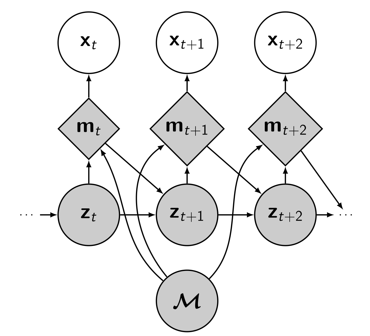 Let us start by defining the components of our model. You can refer to the probabilistic graphical model on the right, too.
Map
The map \(\map\) is a random variable that should reflect the world. In the applications below we focus on 2D environments, so we model \(\map\) as a two-dimensional grid of vector cells, leaving the extension to 3D for future work.
Attention
We additionally identify a sequence of variables \(\chart\Ts\). We call \(\chart\Ts\) charts, and they represent local chunks of content from \(\map\). They are shaped by an attention model \(p(\chart\t \mid \map, \pose\t)\) that extracts content from \(\map\) around the current agent pose \(\pose\t\).
Emission
A neural network with parameters \(\genpars_E\) then takes the chart \(\chart\t\) as input and generates a reconstruction of the current observation \(\obs\t\). This forms the emission distribution \(p_{\genpars_E}(\obs\t \mid \chart\t)\).
Transition
The movement of the agent from time step \(t\) to the next time step \(t + 1\) is modelled by \(p_{\genpars_T}(\pose\tp \mid \pose\t, \control\t)\), where \(\control\t\) is a control input. We implement the transition as a neural network with parameters \(\genpars_T\), similar to the emission model.
The full joint distribution looks like this:
How do we do inference in this model? We decided to use complicated (but differentiable) functions for the attention, emission and transition, so analytical solutions are not easily available. We do not want to linearise either, as that would reduce the expressive power of the model. Luckily, we can use variational inference. Let's call the Evidence Lower Bound (ELBO) to the rescue:
By maximising the ELBO with respect to all model parameters, we are maximising (a lower bound of) the log-probability of the sensor readings \(\obs\Ts\) under the model assumptions. In so doing, we obtain a variational approximation \(q_{\varpars}(\pose\Ts, \map \mid \obs\Ts) \approx p_{\genpars}(\pose\Ts, \map \mid \obs\Ts)\) of the desired posterior, i.e. we are SLAM-ing. SGVB (Kingma and Welling, 2014) allows us to do this with Stochastic Gradient Descent (SGD). Intuitively, the gradients that flow into \(\map\) write content that makes the observations \(\obs\Ts\) probable. Similarly, the poses \(\pose\Ts\) are optimised such that all \(\obs\Ts\) agree with the current map \(q_{\varpars}(\map)\). Our paper (Mirchev et al., 2019) gives the details. Note that the form of the map and attention described in the paper were chosen to illustrate the feasibility of the model in the selected 2D environments. They are by no means final, and we plan to extend them in future work.
We call our model DVBF-LM, which stands for Deep Variational Bayes Filter with a Latent Map.
SLAM in DVBF-LM
Enough with the theory—time to look at some examples. To do SLAM in DVBF-LM we get the approximate posterior \(q_{\varpars}(\map, \pose\Ts \mid \obs\Ts)\). Here is an example of what this looks like in VizDooM, a DooM simulator:
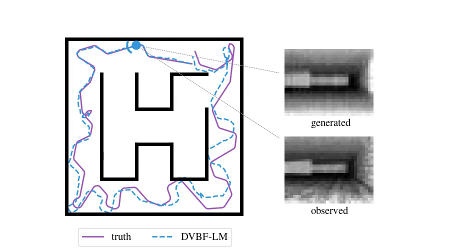
The agent is the VizDooM player. The observations are greyscale images from the player's perspective. On the left, we compare the true player's movement against the mean of \(q(\pose\Ts \mid \obs\Ts)\), the DVBF-LM localisation estimate. As you can see, the agent is aware of its own location and orientation with small errors throughout the whole motion. DVBF-LM can also reconstruct the observed images at any time based on the learned map—visualised on the right. After inference, our model becomes a simulator of the whole environment. So let's use that to our advantage!
Metric maps for navigation
Since DVBF-LM acts as a simulator, we can use it as a proxy for the real world to optimally plan future actions. In the paper we show how the agent can autonomously navigate from one place in a maze to another. This is done through traditional planning algorithms applied on top of the DVBF-LM platform:
The example you see here is bidirectional Hybrid-A* search. On the left, a navigation plan is first constructed based on the learned map. To make this possible, we learn a consistent metric map with the help of a pretrained transition prior (details in the published paper, linked below). On the right, you see the plan executed in the real environment. It works even though the agent has never seen the actual maze map and has no access to its ground truth position in space.
When does uncertainty matter?
Uncertainty is needed whenever we want to quantify confidence in the model estimates. But one other thing it is good for is driving the behaviour of the agent, providing intrinsic motivation. In DVBF-LM we use this to promote the exploration of new, completely unseen environments. We select future controls \(\control\Tsm^*\) that would maximise the information gained about the SLAM map. In simple terms, we query the distributions over observations DVBF-LM would generate for \(\control\Tsm\)—that would be \(p_{\genpars}(\obs\Ts \mid \control\Tsm)\), and then measure the mutual information between these and \(q_{\varpars}(\map)\):
This would not be possible without a probabilistic model.
On the left you can see an agent equipped with laser range finders explore an unknown maze, gradually constructing a map. On the right, we mark the tiles the agent has already visited at least once. This lets us know how effective the exploration strategy is.
TL;DR
- Localisation and mapping can be done both in a fully-probabilistic way and without the need for linearisation.
- We can incorporate learning, making the overall model more flexible.
- Maintaining a metric map estimate (as opposed to a completely abstract one) allows for downstream tasks in the same framework—for example, navigation.
- Map uncertainty is precious—we can use it for exploration.
The described method is not without its problems—in its current form it is slower than traditional SLAM approaches. It also needs to be scaled to real 3D environments. But DVBF-LM is showing promise as a platform for spatial reasoning and we are continuing this line of work at full speed.
Stay tuned!
This work was published at the Robotics: Science and Systems conference, 2019, in Freiburg. We refer to the paper for a more detailed discussion: DOI, preprint.
Bibliography
Hugh Durrant-Whyte, David Rye, and Eduardo Nebot. Localization of autonomous guided vehicles. In Georges Giralt and Gerhard Hirzinger, editors, Robotics Research, 613–625. London, 1996. Springer London. ↩
Diederik P Kingma and Max Welling. Auto-encoding variational Bayes. In Proceedings of the 2nd International Conference on Learning Representations (ICLR). 2014. ↩ 1 2
Atanas Mirchev, Baris Kayalibay, Maximilian Soelch, Patrick van der Smagt, and Justin Bayer. Approximate Bayesian inference in spatial environments. In Proceedings of Robotics: Science and Systems. Freiburg im Breisgau, Germany, June 2019. doi:10.15607/RSS.2019.XV.083. ↩